Implementing and verifying a phase-change solver in OpenFOAM: the one-dimensional Stefan problem

In this post we will discuss how I created a very simple phase-solver. I want to explore and share how we go from defining a problem, deriving some mathematical models and quickly rewrite an existing OpenFOAM solver to add the equations that we have defined. What problem can be relatively simple, but would open more doors once we broaden the scope? The choice was to write a solver to analize the phase change of a metal.

The interesting part of this post is not the solver that works. It is the solver that looked plausible, ran without crashing, that produced easily interpretable data, and that could be validated.

So this is a post about melting, about the math behind it, and mostly about not trusting a simulation until it has earned it.

The problem

Imagine a block of solid against a hot wall. The wall is above the melting point, so the block starts to melt, and a boundary between liquid and solid moves away from the wall over time. I want to know where that boundary is and how fast it moves.

Two things make this harder than ordinary heat conduction.

First, the boundary moves, and I don't know where it is in advance. It is part of the answer, not something I set up at the start. This is what's called a moving boundary or free boundary problem.

Second, melting absorbs energy right at that boundary. Solid does not become liquid for free; it costs the latent heat of fusion, a chunk of energy soaked up at constant temperature. An ordinary heat solver does not know this information.

Away from the boundary, each phase just conducts heat. The heat equation in one dimension is

dT/dt = alpha * d2T/dx2,    alpha = k / (rho * cp)

The two phases are stitched together at the moving front by the energy balance there, the Stefan condition: the heat arriving at the front, minus the heat leaving into the solid, equals the latent heat consumed as the front advances.

The one answer I could check against

For the simplest version, a semi-infinite block initially sitting exactly at the melting temperature, with the wall suddenly raised to a fixed hotter value, there is an exact solution. It comes from a similarity argument: the problem has no built-in length scale, so the temperature profile keeps the same shape over time, just stretched. The front then advances as the square root of time,

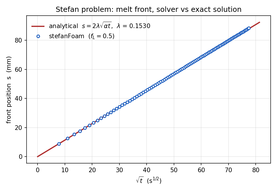
s(t) = 2 * lambda * sqrt(alpha * t)

where lambda is a single number you get by solving one transcendental equation,

lambda * exp(lambda^2) * erf(lambda) = St / sqrt(pi)

and St = cp * dT / L is the Stefan number, the ratio of the sensible heat driving the melt to the latent heat it has to pay. For gallium with a 10 K wall superheat, St comes out around 0.05 and lambda around 0.153.

This is the ruler. Whatever my solver produces, the front it computes has to land on that square-root line. If it does, I believe the solver. If it doesn't, I have a bug.

Building the solver

The plan was to start from laplacianFoam, the stock transient conduction solver, and add three things: a liquid-fraction field, the latent-heat source, and the rule that updates the liquid fraction from temperature.

The liquid fraction, call it fL, is a number in every cell between 0 (solid) and 1 (liquid). The melt front is wherever it crosses 0.5. The energy equation gains a source term that subtracts latent heat as cells melt:

dT/dt = alpha * d2T/dx2 - (L/cp) * dfL/dt

and the liquid fraction is tied to temperature. My first instinct was the obvious one: decide how melted a cell is from where its temperature sits inside a narrow melting band,

fL_target = (T - Tsol) / (Tliq - Tsol)

clamped between 0 and 1, and nudge fL toward that target each iteration with a bit of under-relaxation. Very simple lines. The code compiles, and the simulation runs.

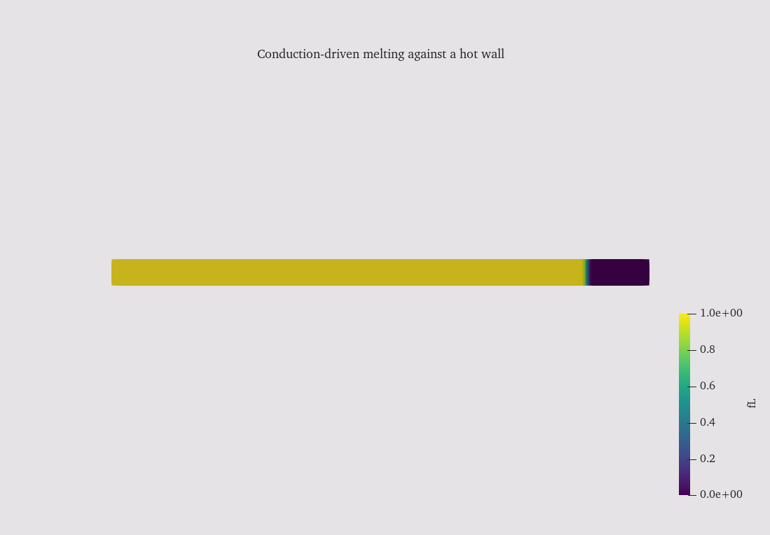
The 1D case in OpenFOAM is a long thin column of cells, one cell thick, with empty boundary conditions on the side faces so the solver treats it as one-dimensional. Wall held hot on the left, everything initialised at the melting point. I ran it, opened the result in ParaView, coloured by fL, and pinned the scale from 0 to 1 so the colours meant something fixed.

The picture that should have stayed two colours

What I expected: solid red where the gallium had melted, solid blue where it hadn't, one sharp line between them sweeping along the strip.

The early frames gave me exactly that. The front grew cleanly out of the wall, two colours, a sharp line, marching the right way. All seemed fine.

I played the timeline, and around timestep 600, I noticed a clear indicator that something needed to be fix. As the run went on,there was no clear separation yet, but the fl numbers jumped around here and there Clearly there is some numerical inaccuracy or something is totally wrong in the derived code itself.

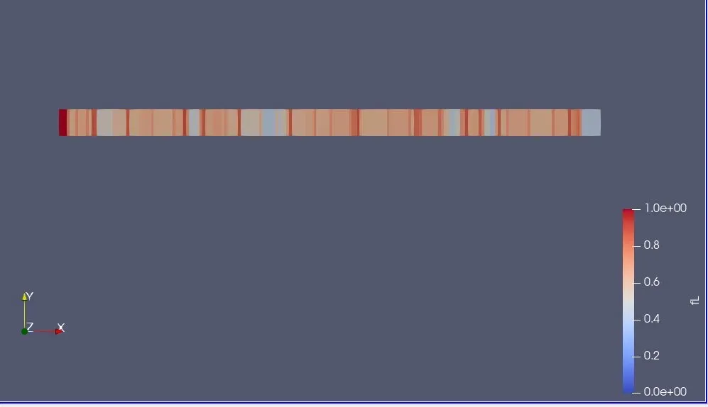
At this point, I opened the data and looking at the numbers

The liquid fraction in the cells behind the front was not random noise. It was sitting at 0.588, almost exactly, over and over.

One number to describe the bug

0.588 was the fingerprint of an oscillation

Here is what was happening. My update blended the old fL with the target at 30 percent:

fL_new = 0.7 * fL_old + 0.3 * fL_target

If a cell is flipping between target 1 and target 0 on alternate passes, that blend doesn't settle in the middle. It converges to a two-step cycle whose upper value is 0.3 / (1 - 0.7^2) = 0.588. Seeing 0.588 told me, to three decimals, that my cells were ping-ponging between fully molten and fully frozen every iteration instead of settling.

The cause is the gain of the coupling between temperature and liquid fraction. With a melting band of width $\Delta T_{\text{band}} = 0.2$ K, the target liquid fraction has sensitivity $\partial f_L^{\text{target}}/\partial T = 1/\Delta T_{\text{band}} = 5\ \text{K}^{-1}$: a temperature perturbation of a few tenths of a kelvin spans the full range of $f_L$. The latent source provides the return path. Melting a cell by $\Delta f_L$ removes latent heat equivalent to a temperature change $\Delta T = (L/c_p)\,\Delta f_L$, and with $L/c_p \approx 210$ K an increment of $\Delta f_L = 0.001$ corresponds to $0.21$ K, exceeding the band width. The round-trip loop gain is therefore

$$G = \frac{\partial f_L^{\text{target}}}{\partial T}\cdot\frac{L}{c_p} = \frac{1}{\Delta T_{\text{band}}}\cdot\frac{L}{c_p} \approx 5 \times 210 \approx 10^{3}.$$

A gain of this magnitude renders the iteration unstable. Under-relaxation at a factor of $0.3$ reduces the effective gain only to $\mathcal{O}(300)$, still far above unity, and no relaxation factor of practical size recovers stability. The scheme is unstable by construction. The clamp of $f_L$ to $[0,1]$ prevents numerical divergence, converting the instability into the bounded oscillation, the speckled field, observed in the solution.

The change of principle

The mistake was letting the update feed back through an arbitrary parameter, the band width, that had nothing to do with the physics. The fix, which is what Voller and colleagues published back in the 1980s, is to feed back through the physics instead.

Instead of reading fL off where T sits in the band, correct fL by how much excess heat the cell actually has above the melting point, converted to melt through the latent heat:

fL_new = clamp( fL + 0.8 * (cp/L) * (T - Tsol), 0, 1 )

The key is the cp/L factor. It is the exact inverse of the L/cp by which fL pushes back on temperature. So the round trip, fL moving T moving fL, now multiplies cp/L by L/cp and the gain cancels to about 0.8, below 1, on purpose, no matter the material or the band width. The cell converts its overshoot into melt, the latent sink pulls the temperature back to the melting point, and it settles. The interface cells end up pinned at exactly the melting temperature, which is the Stefan condition appearing on its own rather than being forced.

One line changed. The principle behind it changed completely.

// broken update: the gain rides on the band width, about 1000
fL = 0.7*fL + 0.3*clamp((T - Tsol)/(Tliq - Tsol), 0, 1);

// fixed update: cp/L cancels the feedback, gain is 0.8 by construction
fL = clamp(fL + 0.8*(cp/L)*(T - Tsol), 0, 1);

The corrected case

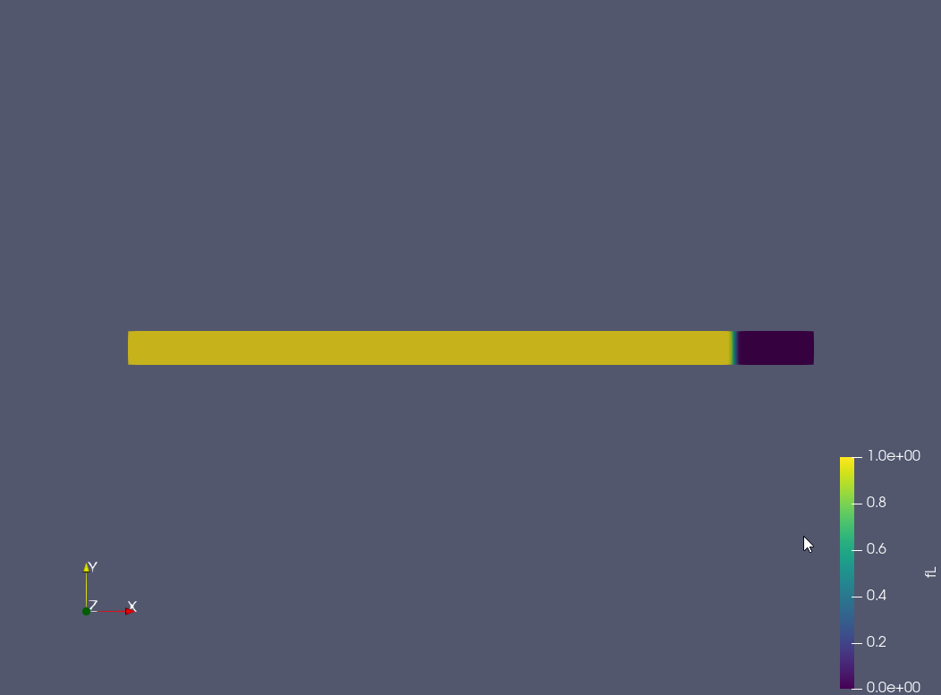
I recompiled, reran, and pulled the numbers again. This time the liquid fraction read 1 behind the front, 0 ahead, with a single cell in between. The temperature fell almost linearly from the wall to the melting point and sat flat in the solid. Exactly the quasi-steady, small-Stefan profile the theory predicts.

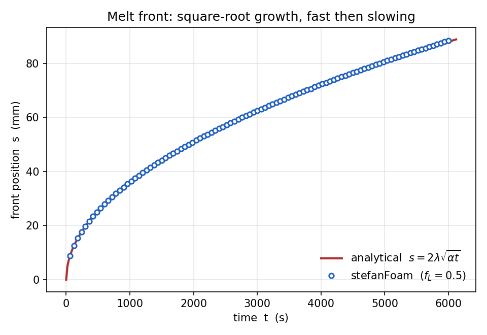
Then the picture: the melt (left) growing from the wall, solid blue solid ahead of it, one clean front marching away and slowing down as it went. The slowing is the square-root law you can see with your eyes.

Did it land on the ruler

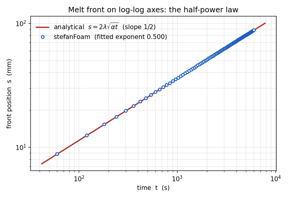
The whole point of the exact solution is that it lets you make a quantitative claim. I extracted the front position, the fL = 0.5 crossing, at every saved time, and plotted it against the square root of time next to the analytical line.

The points sit on the line. Recovering lambda from the slope gives a value within a couple of percent of the analytical 0.153, on the first validated run, before any mesh refinement. On log-log axes the front follows a straight line of slope one half, so the square-root power itself is recovered independently of the coefficient.

Conclusions

The solver itself was straightforward: three additions to a stock conduction solver. The difficulty was diagnostic. The scheme produced a correct-looking front through the first half of the simulation and degraded only later, so a check on the early results alone would have passed it. Two points are worth retaining.

A stable-looking solution can be wrong. The unstable update did not diverge or crash. It produced a physically plausible front for part of the run and broke down progressively, a failure mode that survives a cursory inspection of the field. Validation restricted to the early-time results would have accepted a defective solver.

Field visualisation identifies problems, and quantitative inspection diagnoses them. The contour plot indicated that something was wrong, but it could not have established the loop gain or identified the $c_p/L$ cancellation as the remedy. The constant value of $0.588$ in the liquid-fraction field did both, and only because the field values were examined directly rather than inferred from the colour map. The colour map was the weaker diagnostic; the numbers were decisive.

The next stage extends the same solver to two dimensions with buoyancy, where the melt convects and the interface deforms, and where no analytical solution is available for comparison. The validation against an exact solution is no longer possible, and quantitative verification against benchmark data becomes the only available check. That is the subject of the next post.