A convective melting solver in OpenFOAM: buoyancy-driven melting of gallium

In the previous post we developed a one-dimensional phase-change solver and verified it against the analytical Stefan solution. That case was pure conduction: the melt front advanced with time and remained flat. This was a very simplified case to validate the newly created solver. In reality this is not what happens in a real phase change situation. Once a liquid layer of sufficient depth forms, buoyancy drives convection in the melt, heat is redistributed by the resulting circulation, and the melting front deforms. The melting rate diverges from the conduction prediction, and the problem becomes two-dimensional.

This post extends the solver to fit this more physically accurate regime. Three pieces of physics are added to the conduction plus liquid fraction core: the fluid motion is governed by the incompressible Navier-Stokes equations, the buoyancy force is added with the Boussinesq approximation, and a momentum sink that holds the solid region stationary on the fixed grid. The resulting solver is then verified against the gallium melting experiment of Gau and Viskanta.

A note on validation. In the one-dimensional case an exact analytical solution was available, but no closed-form solution exists for convective melting in a cavity. The verification will be therefore done by comparing the solver results with published experimental and numerical benchmark data.

Governing equations

The liquid is treated as incompressible with constant properties, except in the buoyancy term where the temperature dependence of density is retained. This is exactly the Boussinesq approximation, valid when the relative density variation is small. For liquid gallium with a thermal expansion coefficient $\beta \approx 1.2\times10^{-4}\ \text{K}^{-1}$ and a driving temperature difference of $10$ K, the relative variation is

$$\epsilon = \beta\,\Delta T \approx 1.2\times10^{-3} \ll 1,$$

so the approximation is justified here. The density is linearised about a reference state,

$$\rho(T) = \rho_0\left[\,1 - \beta\,(T - T_0)\,\right],$$

and this variation is retained only in the gravitational term, where it is the sole source of motion, and neglected elsewhere. Absorbing the reference hydrostatic head into a modified pressure $p_{rgh} = p - \rho_0\,\mathbf{g}\cdot\mathbf{x}$, the momentum equation becomes

$$\frac{\partial \mathbf{u}}{\partial t} + (\mathbf{u}\cdot\nabla)\mathbf{u} = -\frac{1}{\rho_0}\nabla p_{rgh} + \nu\,\nabla^2\mathbf{u} - \beta\,(T - T_0)\,\mathbf{g} \;-\; A(f_L)\,\mathbf{u}.$$

The final term, $-A(f_L)\,\mathbf{u}$, is the momentum sink that immobilises the solid; it is constructed in the next section. The energy equation is the one-dimensional balance of the previous post, now with the flow carrying heat as well as conduction:

$$\frac{\partial T}{\partial t} + \nabla\cdot(\mathbf{u}\,T) = \alpha\,\nabla^2 T \;-\; \frac{L}{c_p}\left(\frac{\partial f_L}{\partial t} + \nabla\cdot(\mathbf{u}\,f_L)\right).$$

Reading it term by term: $\partial T/\partial t$ is the local change in temperature, $\nabla\cdot(\mathbf{u}\,T)$ is heat carried by the flow (the new advective term, absent in the conduction case), and $\alpha\,\nabla^2 T$ is conduction. The bracket on the right is the latent-heat sink. The term $\partial f_L/\partial t$ appears because melting a cell, raising its liquid fraction, absorbs latent heat at that rate, removing it from the sensible energy; the factor $L/c_p$ converts that absorbed latent heat into an equivalent temperature change. The companion term $\nabla\cdot(\mathbf{u}\,f_L)$ accounts for liquid fraction transported by the flow, so that latent content advected between cells is also accounted for. In the solid, the momentum sink forces $\mathbf{u}\to 0$, both advective terms vanish, and the equation collapses to the pure-conduction form verified in the previous post: the conduction solver is exactly the zero-velocity limit of this one.

The momentum sink

On a fixed grid the momentum equation is solved in every cell, including those that are fully solid, where the fluid must not move. A body force is therefore added that is negligible in liquid and overwhelming in solid. The standard construction treats the partially-melted cell as a porous medium whose porosity is the liquid fraction $f_L$: fully liquid ($f_L = 1$) means fully open, fully solid ($f_L = 0$) means closed. Modelling the flow resistance of such a medium with the Carman-Kozeny relation for permeability gives the sink coefficient

$$A(f_L) = C\,\frac{(1 - f_L)^2}{f_L^{3} + q}.$$

The behaviour at the two limits is what matters. In a fully liquid cell the numerator $(1-f_L)^2$ vanishes, so $A = 0$ and the momentum equation is untouched. As $f_L \to 0$ the denominator collapses and $A$ grows without bound, producing a force large enough to drive the velocity to zero and hold the solid stationary. The small constant $q \approx 10^{-3}$ prevents division by zero in fully solid cells. The constant $C$ sets the strength of the penalty; for a pure substance the mushy region is numerically thin and $C$ is a numerical parameter rather than a material property, chosen large enough to immobilise the solid without making the system ill-conditioned.

Dimensionless parameters

The solver works in dimensional SI units: the real viscosity, expansion coefficient, gravity and diffusivity are supplied directly, and no dimensionless number is entered anywhere. The groups below are therefore not inputs to the computation. They serve two purposes: they identify the flow regime, which is what allows this case to be compared with other studies of the same problem, and the Stefan number sets the time-scaling used later in the benchmark comparison.

They arise when the governing equations are written in non-dimensional form. Scaling lengths by the cavity height $H$, velocity by the thermal diffusion speed $\alpha/H$, time by $H^2/\alpha$, and temperature by the wall difference $\Delta T$, and substituting into the momentum and energy equations, three coefficients remain in front of the terms once the equations are divided through. These are the governing groups:

$$\mathrm{Pr} = \frac{\nu}{\alpha},\qquad \mathrm{Ra} = \frac{g\,\beta\,\Delta T\,H^{3}}{\nu\,\alpha},\qquad \mathrm{St} = \frac{c_p\,\Delta T}{L}.$$

Each is the ratio that survives in front of a particular term. The Prandtl number, multiplying the viscous term, is the ratio of momentum diffusivity to thermal diffusivity. The Rayleigh number, multiplying the buoyancy term, measures the strength of buoyant driving against the two diffusive processes that damp it. The Stefan number, appearing in front of the latent term in the energy equation, is the ratio of sensible heat to latent heat. For the gallium case,

$$\mathrm{Pr} \approx 0.021,\qquad \mathrm{Ra} \approx 6\times10^{5},\qquad \mathrm{St} \approx 0.04,$$

which places the problem in the regime of laminar convection in a low-Prandtl-number liquid metal. The low Prandtl number is the one of practical consequence for the discretisation: since $\mathrm{Pr} = \nu/\alpha \ll 1$, momentum diffuses far more slowly than heat, and the velocity boundary layer on the hot wall is correspondingly thinner than the thermal layer, by a factor of order $\sqrt{\mathrm{Pr}}$. The mesh must resolve that thin velocity layer, which is finer than the temperature field alone would demand, and under-resolving it weakens the computed convection. This is the reason the mesh is refined towards the hot wall.

Solver construction

The solver, here named meltFoam, is built from buoyantBoussinesqPimpleFoam, the stock transient solver for buoyant incompressible flow. This base already provides the incompressible Navier-Stokes equations, the Boussinesq buoyancy term through the modified pressure $p_{rgh}$ and the kinematic density $\mathrm{rhok} = 1 - \beta(T - T_{ref})$, and the PIMPLE algorithm for pressure-velocity coupling. The phase-change physics is added through three localised modifications, paralleling the one-dimensional build.

First, the liquid-fraction field and the phase-change constants are declared, together with the Carman-Kozeny coefficient field $A(f_L)$. Second, the momentum sink is added to the velocity equation as an implicit term:

fvVectorMatrix UEqn
(
    fvm::ddt(U) + fvm::div(phi, U)
  + turbulence->divDevReff(U)
  + fvm::Sp(Darcy, U)
 ==
    fvOptions(U)
);

The implicit treatment, fvm::Sp, places the sink coefficient on the matrix diagonal. In solid cells this coefficient is of order $10^{6}$, and an explicit treatment of a term that large would destabilise the solution; on the diagonal it instead dominates the row and drives the velocity to zero. Third, the energy equation is solved with the latent source and the liquid-fraction update iterated to consistency:

for (int phaseIter = 0; phaseIter < 10; ++phaseIter)
{
    fvScalarMatrix TEqn
    (
        fvm::ddt(T) + fvm::div(phi, T)
      - fvm::laplacian(alphaEff, T)
     ==
      - (L/cp)*(fvc::ddt(fL) + fvc::div(phi, fL))
    );
    TEqn.solve();

    fL = min(scalar(1), max(scalar(0), fL + 0.8*(cp/L)*(T - Tsol)));
}

Darcy = Cu*sqr(scalar(1) - fL)/(pow3(fL) + qCK);
rhok  = 1.0 - beta*(T - TRef);

The liquid-fraction update is the same stable correction derived and verified in the one-dimensional case; the addition of convection does not alter it. The latent source now also carries the advected component $\nabla\cdot(\mathbf{u}\,f_L)$. After the phase loop, the Carman-Kozeny coefficient and the buoyancy density are refreshed from the updated temperature and liquid fraction, so that the subsequent momentum and pressure solves act on the current solid distribution and buoyancy field. Because the energy equation is solved within the PIMPLE outer loop, these couplings are iterated together several times per time step.

Case configuration

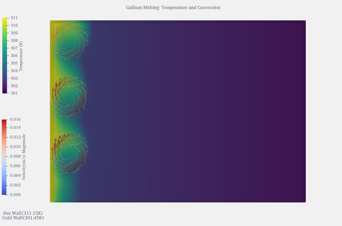
The case reproduces the configuration of Gau and Viskanta: a rectangular cavity $88.9$ mm wide and $63.5$ mm high, with the left wall held at $311.15$ K, above the melting point, and the right wall at $301.45$ K, below it. The horizontal walls are adiabatic and gravity acts downward. The gallium is initially solid at the cold-wall temperature, and melting proceeds from the heated left wall.

The domain is discretised with a $160 \times 120$ mesh, graded in the horizontal direction so that cells are clustered towards the hot wall: the cells there are roughly $0.26$ mm wide, narrowing from about $1.0$ mm at the cold wall. This grading is motivated by the low Prandtl number, which makes the velocity boundary layer on the hot wall considerably thinner than the thermal layer; a uniform mesh of comparable cell count under-resolves that layer and weakens the computed convection. The time step is adaptive, limited by a maximum Courant number of $0.9$. Velocity uses no-slip conditions on all walls, and the pressure uses a fixed-flux condition consistent with the buoyancy-driven formulation.

One practical note on the linear solver. The Carman-Kozeny sink produces a pressure matrix whose coefficients vary by roughly six orders of magnitude across the solid-liquid interface, which makes the pressure equation stiff. A geometric-algebraic multigrid (GAMG) solver reduces the iteration count per pressure solve from order $10^{2}$, with a preconditioned conjugate gradient method, to single digits, and is strongly preferable for this problem; it roughly halves the total run time.

Results

The computed flow develops as expected for side-heated convective melting. Liquid adjacent to the hot wall is heated, rises under buoyancy, travels along the top of the cavity, and descends along the melt front, establishing a single clockwise circulation cell. This circulation transports heat preferentially to the upper part of the front, which therefore advances faster than the lower part, producing the characteristic forward-leaning interface.

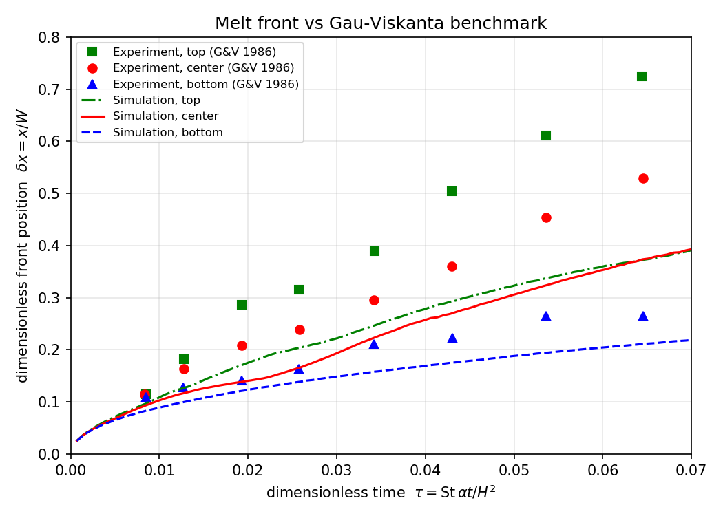
The solver agrees with the experimental data only at early times: for $\tau \lesssim 0.02$ the computed fronts at all three heights track the experimental points closely, and the correct ordering is reproduced, with the top of the front advancing fastest and the bottom slowest, but at later times the computed fronts lag the experiment, increasingly so as $\tau$ grows, with the top and centre curves falling below the measured positions while the bottom curve remains closer.

This lag is not removed by some tweakings. The computation was repeated with the Carman-Kozeny constant reduced from $10^{6}$ to $10^{5}$ and with the mesh refined and graded towards the hot wall, the two changes most likely to strengthen the computed convection. Neither closed the gap in a noticeable way. Within the range tested, the front position is insensitive to these parameters, which indicates the lag is not simply an artefact of the mushy-zone penalty strength or of under-resolution of the velocity boundary layer.

The lag therefore appears to originate in the model rather than in its numerical settings. This conclusion is sharpened by an important external reference point: the same benchmark, computed with the Lethe finite-element solver, reproduces the Gau and Viskanta front positions closely, including at the later times where the present solver lags. Since another implementation of essentially the same physics matches the experiment, the discrepancy cannot be attributed to the way that i wrote the solver itself, nor to a fundamental limitation of the enthalpy-porosity approach. It must lie in a specific modelling choice in which the two solvers differ.

Hypotheses and next steps

The two solvers differ in several respects, each a candidate explanation for the later-time lag, and the natural next step is to vary these one at a time and identify which closes the gap.

The main hypothesis is the treatment of the solid region. The present solver immobilises the solid with a Carman-Kozeny Darcy sink, a momentum force proportional to velocity that grows as the liquid fraction falls. The Lethe computation instead uses a variable viscosity that rises sharply from the liquid to the solid value. These two mechanisms damp the near-interface flow differently, and the Darcy sink may suppress convection in the partially-melted cells more than the viscosity formulation does, which would reduce the heat carried to the upper front and produce exactly the observed lag. Reproducing the viscosity-based treatment in the present solver, and comparing, is the first test.

The second hypothesis is mesh strategy. The reference computation uses adaptive refinement that concentrates cells at the moving front and the walls at every step, whereas the present mesh is static and graded only towards the hot wall. If the convection is sensitive to resolution at the front itself, rather than only at the hot wall, a static mesh may under-resolve it as the front advances into the coarser interior. Repeating the computation with refinement tracking the front would test this.

A third possibility is the strength of the convection-melting coupling within each time step: how tightly the momentum, energy and liquid-fraction updates are converged together before advancing. Under-converged coupling would weaken the effective convection. This can be examined by tightening the outer-iteration count and tolerances and confirming whether the front position responds.

What appears to be the biggest culprit here though is how we implemented the Darcy sink. Changing this could have a greater effect rather than doing adaptive refinement

The conclusion therefore is the following: The solver reproduces the correct flow structure and the conduction-to-convection transition, and agrees with experiment while the flow is conduction-dominated. It under-predicts the melting rate at later times, by a margin that is robust to the mushy-zone constant and the hot-wall mesh resolution. Because an independent solver matches the same benchmark, the lag is a property of a modelling choice in the present implementation, and the most likely candidate is the Darcy momentum sink. Identifying the responsible choice is the subject of the next stage of this work.