Marangoni-driven weld pool solver in OpenFOAM: moving arc welding of stainless steel

Introduction
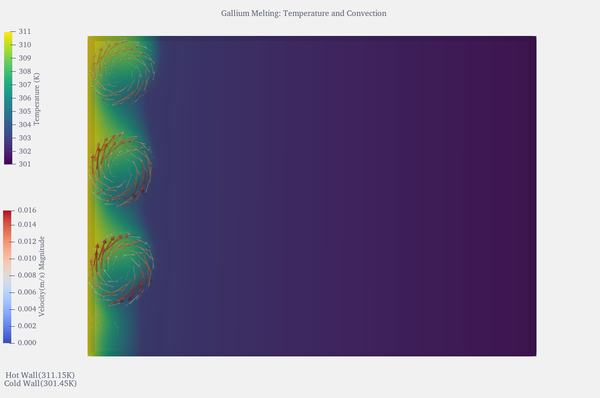
The next step that follows the 2D buoyancy-driven melting of gallium is of course analyzing a 3D case and adding more physics to the solver.
The question that we want to answer now is, how can we simulate a moving heat source, such as the tip of a tig weld, and what physical properties can we include, and which we can exclude for now, to have a basic, quantifiable and measurable data that can be useful for a simulator to solve?
Of course, this means going step by step, and deciding good tradeoffs between simplification of the model, time of delivery, set up and simulation time.
Keeping these factors in mind, weldFoam was created to answer the following questions:
What shape will my welding liquid metal pool have, for a specific power and speed setting?
To answer this accurately, the following assumptions and physical properties will be included:
Surface tension changes due to phase and temperature changes, viscosity , shape of the heat source ( it is not a simplified boundary wall anymore, but a moving source of heat, with its own shape ), and properties of the metal.
The governing equations
The pool is an incompressible liquid metal, driven by density differences from temperature, solved transiently, and coupled to a temperature field.
buoyantBoussinesqPimpleFoam . shipped already in OpenFoam, serves this purpose, and the gallium melting solver from the previous post was already built on it.
This is the energy equation, which has temperature as a passive scalar
$$\frac{\partial T}{\partial t} + \nabla\cdot(\mathbf{u}T) = \nabla\cdot(\alpha\,\nabla T)$$
with $T$ the temperature, $\mathbf{u}$ the velocity, and $\alpha$ the thermal diffusivity, a single lumped property describing how fast heat spreads. That works when heat is only carried by the flow and conducted through the metal.
This is not sufficient to model the melting process, $\alpha$ hides the individual material properties inside one number, which in our case , it is not constant.
Four material properties are needed to write the version we want:
- $\rho$, density, in kilograms per cubic metre
- $c_p$, specific heat: the energy needed to warm one kilogram by one kelvin
- $k$, thermal conductivity: how readily heat flows down a temperature gradient
- $L$, latent heat of fusion: the energy needed to melt one kilogram, with no temperature change
The lumped diffusivity above is just $\alpha = k/\rho c_p$ (conductivity divided by density times specific heat)
The product $\rho c_p$ converts a temperature into an energy per cubic metre, so multiplying the whole equation by it makes our units into watts, so that we can add the heat source ( the tig power ) directly.
One more field is needed to describe whether a cell is liquid or solid , or somewhere in between. Each cell is assigned a liquid fraction $f_L$, running from 0 for fully solid to 1 for fully liquid. Solid and liquid share the same mesh, and $f_L$ records how much of each is present in a given cell.
With those defined, here is what weldFoam solves:
$$\rho c_p \left( \frac{\partial T}{\partial t} + \nabla\cdot(\mathbf{u}\,T) \right) = \nabla\cdot(k\,\nabla T) - \rho L \left( \frac{\partial f_L}{\partial t} + \nabla\cdot(\mathbf{u}\,f_L) \right) + q_{arc}$$
In words: the heat stored in a bit of metal changes because the flow carries heat in and out, heat conducts through the faces, melting absorbs some of it, and the arc is adding more.
The left side is the heat stored, and how it moves with the metal. $\partial T/\partial t$ is a fixed point in the plate getting hotter or colder. $\nabla\cdot(\mathbf{u}T)$ is heat arriving because liquid flowed in carrying it. In the solid that second term is zero, since nothing moves. In the pool it dominates, and it is the term the Marangoni flow acts on: the surface flow is how the arc's heat reaches the pool edge.
$\nabla\cdot(k\nabla T)$ is conduction. Heat runs down the temperature gradient at a rate set by $k$, and the divergence is the net amount arriving in the cell. In a solid this is the only way heat moves, and on its own it gives a pool that is deeper and narrower than the real one. The difference between the two is the whole story of this post.
$\rho L(\partial f_L/\partial t + \nabla\cdot(\mathbf{u}f_L))$ is the latent heat. Melting absorbs energy without raising the temperature, because it goes into breaking the crystal structure rather than into making atoms vibrate faster. The bracket is how fast a cell is melting, plus how much already-melted metal flowed in from elsewhere. The minus sign is because this energy comes out of the heating budget. For 316L, melting a kilogram costs the same energy as heating it by about 400 K, so it is not a small correction.
$q_{arc}$ is the arc, in watts per cubic metre.
The Marangoni boundary condition
Surface tension is a phenomenon that we need to take into account, as it alters the shape and inner flow of the liquing. For this liquid metal, the tension gets weaker as the metal gets hotter.
On the melting pool surface the temperature is the highest under the arc and gets lower toward the edge. So the surface tension is weakest at the centre and strongest at the rim, therefore the liquid is pulled away towards the edge.
This behavior of course does not occur only at the surface. The surface layer pulls on the liquid immediately below it, and the liquid resists through its viscosity. The two balance, and that balance is what determines how fast the surface actually moves. Writing it down needs three quantities: the surface tension $\sigma$ and how it changes with temperature, $d\sigma/dT$; the dynamic viscosity $\mu$; and the velocity component parallel to the surface, $\mathbf{u}_t$.
The pull is $\frac{d\sigma}{dT}\nabla_t T$, where $\nabla_t T$ is the sideways part of the temperature gradient, the part surface tension can act on. The liquid resists being sheared and pushes back with a stress $\mu\,\partial\mathbf{u}_t/\partial n$, where $n$ points into the metal. That same stress, read the other way round, is what the surface exerts on the liquid below, which is how the motion spreads downward. At the surface the two balance:
$$\mu \frac{\partial \mathbf{u}_t}{\partial n} = \frac{d\sigma}{dT}\,\nabla_t T$$
For the 316L used here, with low sulfur and oxygen, $d\sigma/dT$ is about $-0.36\times 10^{-3}$ N/m/K.
We can see here that it is a negative value, hence the flow runs outward from the centre, carrying the arc's heat sideways to the pool edge instead of letting it conduct downward. That gives a wide, shallow pool. A different steel, or the same steel with more dissolved oxygen, could have a different sign and produces a different shape.
What was added to the solver
The moving arc
The heat input is a Goldak double ellipsoid, the standard arc model: a Gaussian distribution with a different length ahead of and behind the arc, so the deposited energy trails backward the way a real arc does. It is parametric, and the parameters are the arc's physical dimensions.
What matters for the implementation is that none of it is in the solver. It is an fvOption, which is OpenFOAM's mechanism for adding a source term to an equation at runtime, from a dictionary. The solver's energy equation ends with
+ fvOptions(rhoCp, T)and that single line is the entire coupling. At each time step the framework asks every registered option to add its contribution to the matrix. If system/fvOptions is empty, the term is zero and the solver runs as pure conduction and convection. The arc is configured entirely here:
goldak
{
    type            movingGoldakSource;
    active          true;

    power           1500;           // [W] gross arc power
    efficiency      0.8;            // [-] fraction reaching the plate

    a               0.003;          // [m] half-width across the weld
    b               0.001;          // [m] depth into the plate
    cFront          0.003;          // [m] length ahead of the arc
    cRear           0.006;          // [m] length behind the arc

    startPosition   (0.008 0 0.012);
    direction       (1 0 0);
    speed           0.005;          // [m/s] travel speed
}
Three consequences follow from doing it this way.
- The sweep is a scripted edit, not a recompile. Changing power and travel speed across a parameter study is
foamDictionary -entry goldak/power -set 2000, and the same solver binary runs every case. - Turning the arc off is
active false, which gives a conduction-only run for comparison with no other change to the setup. That is how the verification runs below are built. - And the source is a separate compiled library, loaded by name in
controlDict:
libs (movingGoldakSource marangoniBC);so it can be replaced with a different heat source model, a laser or a stationary arc, without touching weldFoam at all.
One parameter is worth a note. The depth $b$ sets how far into the plate the energy is deposited. An arc heats the surface, so it should be small. An early run used 3 mm, spreading the power through three millimetres of metal, and produced a pool that was too cold and too small. At 1 mm the power lands where it should.
The Darcy sink
Solid and liquid share one mesh, so something has to stop the solid moving. The standard trick is a force that grows as a cell solidifies, strong enough to hold it still. The usual form scales it by a constant you choose, and choosing it is a nuisance: too small and the solid creeps, too large and the matrix becomes ill-conditioned.
Instead the coefficient comes from the microstructure. A solidifying alloy grows dendrites, and the liquid trapped between them flows as through a porous medium whose pore size is the dendrite arm spacing. That gives a permeability, and the drag follows from it:
$$A(f_L) = \frac{180\,\nu}{\lambda_2^{2}}\,\frac{(1 - f_L)^2}{f_L^{3}}$$
with λ2=10 μm for 316L at welding cooling rates. The practical difference is that this is a material property rather than a tuning knob: the same value carries to any other 316L case without adjustment.
The Marangoni boundary condition
Two things have to be true at the pool surface: liquid is pulled sideways by the surface tension gradient, and no liquid crosses the surface. The first is the physics of the previous section. The second sounds trivial and is where the first attempt failed.
That attempt used codedMixed, blending between a fixed velocity and a fixed gradient according to the local liquid fraction. It leaked. The cumulative continuity error grew steadily with one sign, and the minimum temperature in the domain drifted from 300 K down to 82 K, which is what you see when fluid crosses a boundary that should be closed. The cause is structural: a mixed condition that has blended fully to the gradient side no longer constrains the wall-normal component at all.
The replacement is a port of the AdditiveFOAM condition to v2212, built on transformFvPatchVectorField. That base class exists for exactly this case, where the normal and tangential directions need different treatment. Two pieces of OpenFOAM vocabulary make the code readable:
- patchInternalField() is the velocity in the cell immediately behind each boundary face.
- deltaCoeffs() is one over the distance from that cell centre to the face, so multiplying a velocity difference by it gives a gradient.
- I - sqr(nHat) is the projector onto the surface: applied to a vector, it strips out the component pointing through the surface and leaves the part lying in it.
The class provides two hooks. The first, evaluate(), sets the velocity on the face itself:
// Pure slip: tangential part of the adjacent cell velocity,
// normal component identically zero.
vectorField::operator=(transform(I - sqr(nHat), pif));
The face velocity is the neighbouring cell's velocity with the through-surface component removed. Nothing can leak, because the normal velocity is zero by construction rather than by a coefficient that happens to be large.
The second hook, snGrad(), is the one the momentum equation actually uses. It supplies the velocity gradient at the boundary, which is where the Marangoni stress enters:
return
(
    transform(I - sqr(nHat), pif) - pif                         // kill the normal component
  + coeff*transform(I - sqr(nHat), tGrad)/patch().deltaCoeffs() // impose the tangential shear
)*patch().deltaCoeffs();
The first line is the tangential part of the cell velocity minus the whole of it, which is just minus the normal component; multiplied by deltaCoeffs it becomes the gradient that drives the normal velocity to zero at the face. The second line is $\frac{1}{\mu}\frac{d\sigma}{dT}\nabla_t T$ from the previous section, projected into the surface. coeff is that ratio, computed once from the dictionary.
Placing the stress here rather than in a prescribed face value is what makes it work. snGrad() feeds the diffusion term of the momentum matrix, so the shear is part of the linear solve rather than a number imposed afterwards, and it stays stable at the temperature gradients under an arc.
One guard, not physics: the temperature is capped before the gradient is taken, so a single cell overshooting in a transient cannot inject an enormous stress. The cap sits at 3000 K and the run peaked at 2316 K, so it never engaged.
Case configuration
The case is a bead-on-plate weld on SS316L, half of the plate meshed with a symmetry plane on the weld centreline. The domain is 50 mm along the weld, 15 mm across from the centreline, and 12 mm deep, sized so that a 4.5 s run at 5 mm/s keeps the pool inside the region of uniform mesh and the heat does not reach the far walls.
| Setting | Value |
|---|---|
| Material | SS316L, ORNL AdditiveFOAM set: 7955 kg/m3, k 25 W/m K, cp 675 J/kg K, L 268 kJ/kg, μ 2.2 mPa s, Tsol 1471 K, Tliq 1709 K, λ2 10 µm |
| Marangoni | $d\sigma/dT = -0.36\times 10^{-3}$ N/m/K |
| Arc | Goldak, 1500 W at 0.8 efficiency, 1200 W net; a 3 mm, b 1 mm, cfront 3 mm, crear 6 mm; 5 mm/s |
| Mesh | 731,000 cells, 0.125 mm isotropic over 6 mm half-width and 4 mm depth along the weld corridor, graded to about 2 mm in the far field |
| Boundary conditions | Marangoni slip on the top surface, no slip elsewhere; top adiabatic, plate ends zero gradient, far side and bottom held at 300 K |
| Time | Adaptive, Courant number 0.5, maximum step 5 ms; 4.5 s of weld |
The mesh resolution was set from the physics rather than a cell count. A Rosenthal estimate at this power and speed gives a pool about 3 mm wide and 2.6 mm deep, and the 238 K mushy band is about 1.2 mm thick at the gradients under the arc. At 0.125 mm that is roughly 20 cells across the pool depth and 9 or 10 through the mushy band. Earlier runs on a coarser mesh resolved the band by half a cell, and the solidification front was a staircase.
The run is 6 ranks with Scotch decomposition. The case is meshed with blockMesh, decomposed, and launched in the background so it survives the terminal:
blockMesh && checkMesh
decomposePar
nohup mpirun -np 6 weldFoam -parallel > log.weldFoam 2>&1 &
Once the pool is developed the Courant limit at 0.125 mm and 0.3 m/s puts the time step near 0.15 ms, and 4.5 s took about 24 hours of wall time on a desktop. Fields are written every 0.1 s in binary; the first attempt wrote every 25 ms in ASCII and filled the disk before it finished.
A note on what made the case work. The version that produced the result below came after several that did not, and each failure was one specific thing: the mesh grading inverted so the fine cells were at mid-depth; the isothermal liquid-fraction update on an alloy; the leaking mixed boundary condition; and the Goldak depth three times too large. Each was found by checking one number against what the physics said it should be: the fraction of input power appearing as sensible heat, the sign of the cumulative continuity error, the minimum temperature in the domain.
None of the failed runs crashed the solver. Each produced a pool that was plausible at a glance and wrong on inspection.
Results
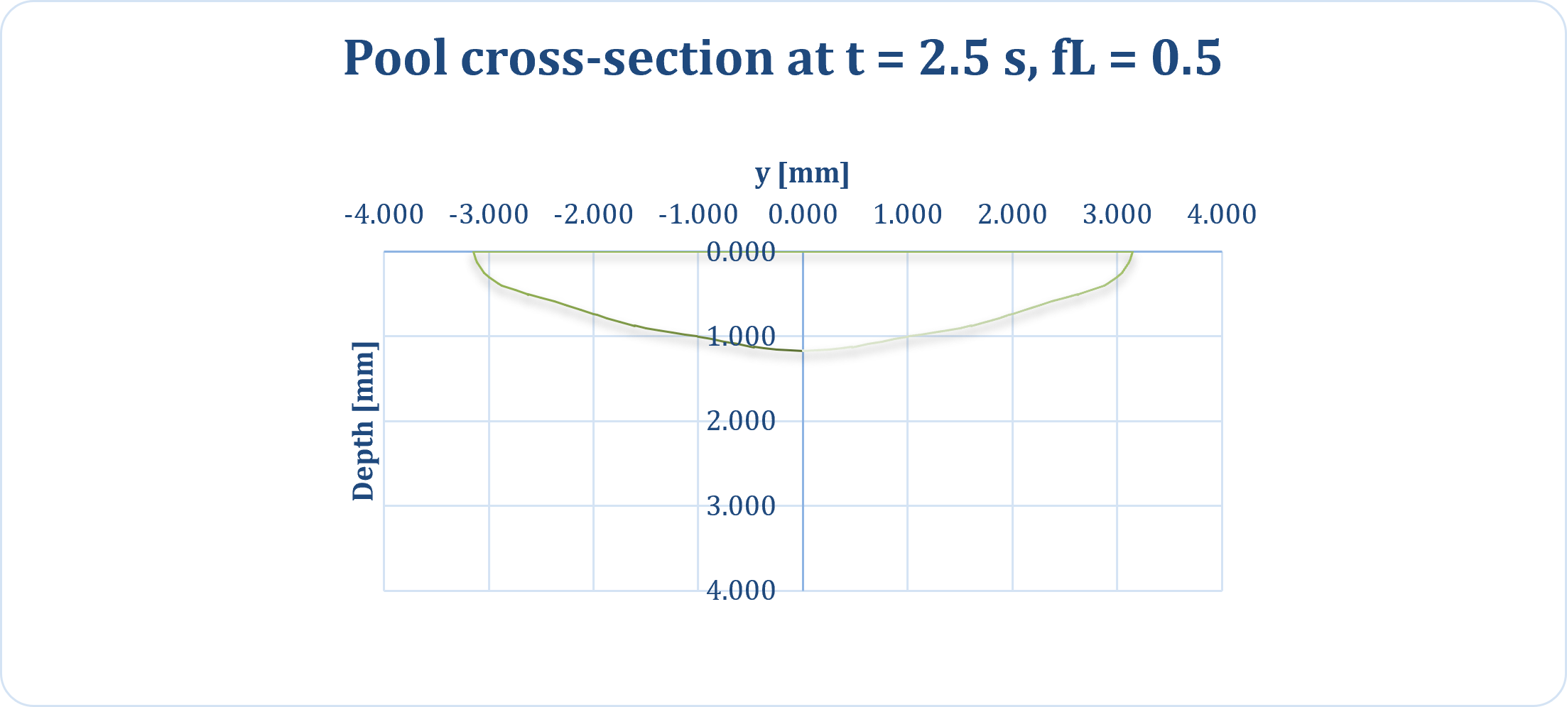
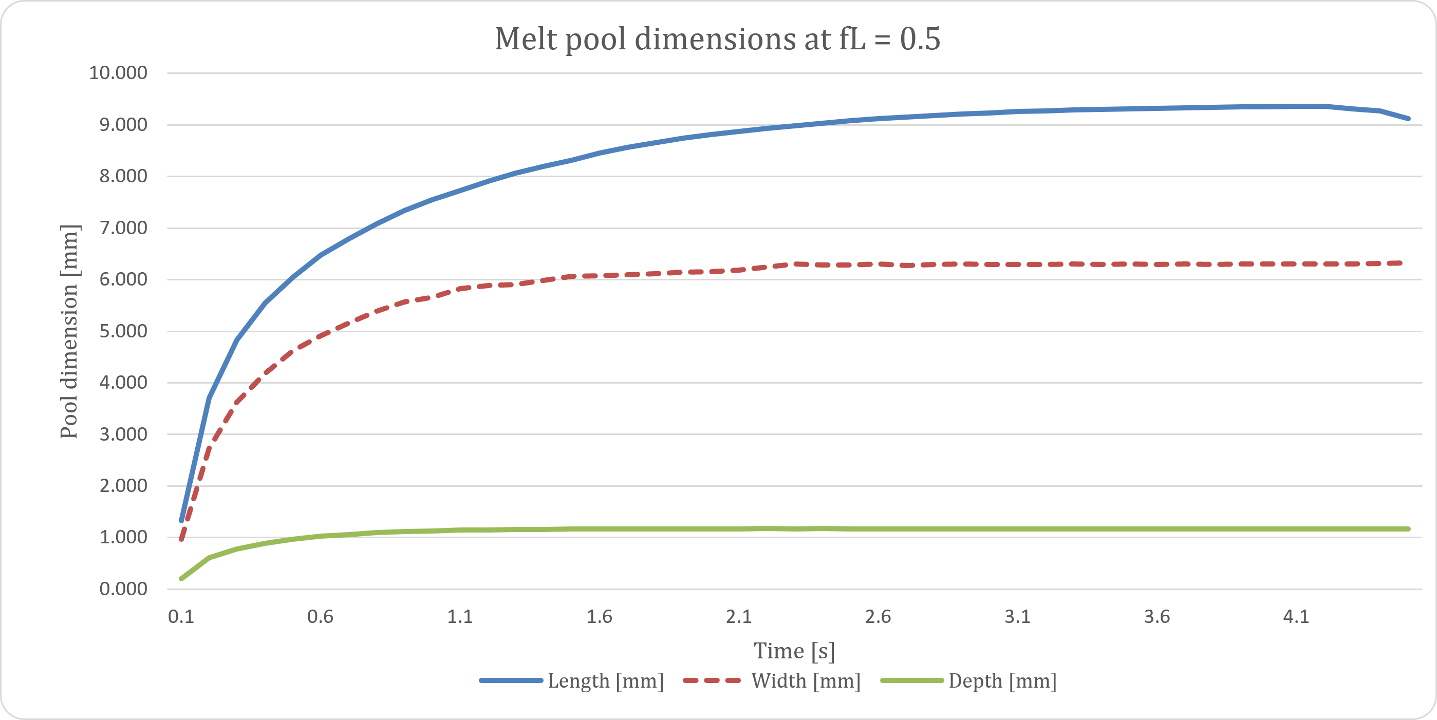
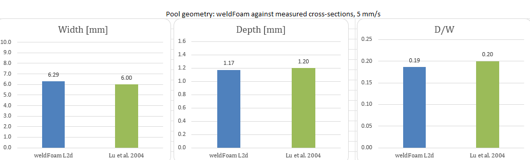
The pool reaches a quasi-steady state about 1.5 s after the arc starts. After that its dimensions hold constant to within a percent. At 2.5 s it is 6.3 mm wide, 1.2 mm deep and about 9 mm long, giving a depth-to-width ratio of 0.19.
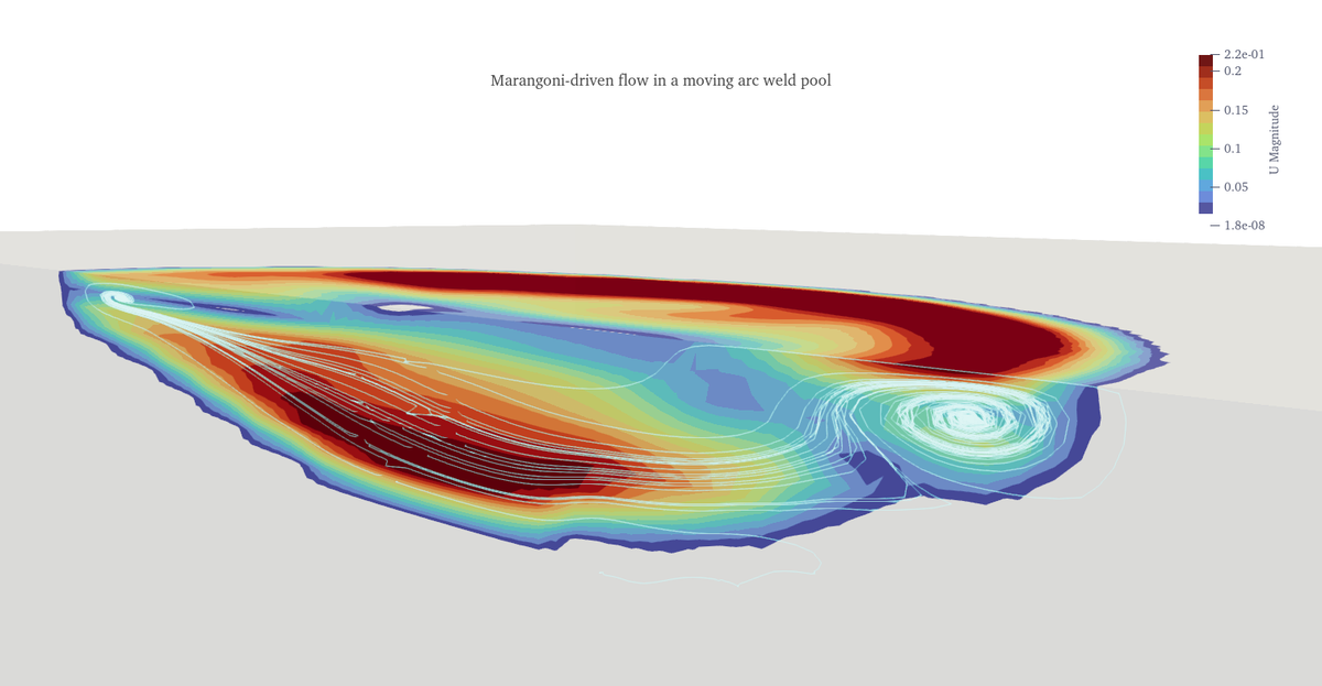
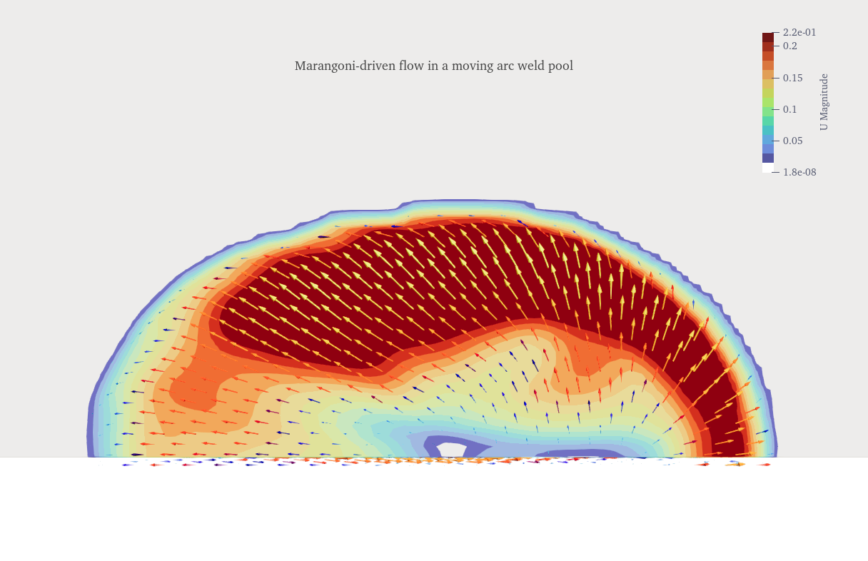
The peak temperature is 2316 K, on the centreline just behind the arc. The maximum velocity is 0.31 m/s, in the surface layer about 2 mm off the centreline and 3.5 mm behind the arc, where the surface temperature gradient is steepest.
There are three recirculation cells. The main one fills most of the pool: the surface flow runs outward and rearward from the arc, turns down at the pool edge, and returns forward along the bottom. A smaller counter-rotating cell sits under the arc at the front of the pool, where the forward surface flow meets the advancing solidification front. A third, weaker one forms at the trailing edge.
The velocities are an order of magnitude below what a laser pool reaches at the same power. An arc spreads the same energy over a footprint about ten times larger, so the surface temperature gradients are that much gentler.
Benchmark
Lu, Fujii and Nogi (Scripta Materialia 51, 2004, 271–277) welded bead-on-plate tracks on SUS304 stainless steel with a moving gas tungsten arc at 160 A, 3 mm electrode gap, and travel speeds from 0.75 to 5 mm/s, then sectioned and etched the beads to measure the pool.
Their low-oxygen shielding gas (Ar with 0.1 vol% O2) gives a weld metal oxygen content of a few tens of ppm. That is below the level at which $d\sigma/dT$ changes sign, so the flow in their pools runs outward, the same regime as this simulation.
Their 5 mm/s case matches the travel speed used here. They report a depth-to-width ratio of about 0.2 across the full speed range for this gas, and the width at 5 mm/s reads as about 6 mm from their published cross-sections.
| Quantity | Lu et al. 2004, 5 mm/s | weldFoam, 5 mm/s |
|---|---|---|
| Width | ≈ 6 mm | 6.3 mm |
| Depth | ≈ 1.2 mm (implied) | 1.2 mm |
| Depth / width | ≈ 0.2 | 0.19 |
Four differences between the experiment and the simulation are worth stating. The experiment is on SUS304 and the solver uses an SS316L property set. Both are austenitic stainless with similar thermal behaviour, but their liquid viscosity is about three times the value used here. The arc power is reported as a current with no voltage, so the net heat input is an estimate, of order 1300 to 1400 W against the 1200 W simulated. The simulated surface is flat and the real one is not. And the width at 5 mm/s is read from a photograph rather than a table.
The depth-to-width ratio is the most reliable of the three numbers, since it does not depend on the arc efficiency.
Conduction alone, at this heat input, gives a pool about half the width and twice the depth. The wide shallow shape the experiment shows comes from the outward Marangoni flow, and the solver reproduces it using the material's own $d\sigma/dT$ with no tuning.
What this is useful for
The benchmark shows the physics and the implementation are correct at this operating point. That is what the comparison is for, and it is as far as it goes.
The solver itself predicts penetration depth. Measuring penetration normally means sectioning and etching a coupon, and the solver gets it from material properties rather than from a fitted correlation, so it can be run at parameter combinations nobody has cut a coupon for.
A surrogate model fitted to a sweep over power and travel speed would make that prediction instant instead of a day of compute per point. A robot cell programmer could use it to check whether a proposed power and speed will reach the required penetration on a given thickness.
That last step is a first-pass check. It is valid only inside the range it was trained on, for that material and thickness, and it carries every limitation listed below. It reduces how many coupons you cut, not whether you cut them.
Limitations and next steps
Four assumptions limit what this model can be used for.
The surface is flat. In a real arc weld the arc pressure depresses the pool and surface tension shapes the bead. Neither is modelled here.
The flow is laminar. At the Reynolds number of this pool, around a thousand, that holds. At higher power it does not.
$d\sigma/dT$ is a constant. In a steel with dissolved oxygen or sulfur it changes sign at a temperature that depends on the concentration, so a real pool can have inward flow at the centre and outward flow at the rim at the same time.
The electromagnetic body force from the welding current is not included. At 160 A it is smaller than the Marangoni stress, but it is not zero.
Two verification runs follow directly from this one. The first is the sign flip, $d\sigma/dT = +0.36\times 10^{-3}$, which should produce the deep narrow pool of the high-oxygen case in the same paper. The second is the same case run in AdditiveFOAM, which shares the material data and the boundary condition, giving a code-to-code check on the implementation.
After that the case becomes the reference point for a parameter sweep over power and travel speed, from which a surrogate model of pool geometry can be fitted. The solver then moves to a deformable free surface.
Code
weldFoam, the Goldak arc source and the Marangoni boundary condition are at github.com/KabLov92/eigenflow_solvers, GPLv3.
The SS316L property set and the Marangoni boundary condition are taken from ORNL's AdditiveFOAM, also GPLv3, and the boundary condition was ported to OpenFOAM v2212. The Goldak arc source, the implicit latent-heat treatment and the solver itself are new.
References
- D. Rosenthal. The theory of moving sources of heat and its application to metal treatments. Transactions of the ASME 68 (1946) 849.
- J. Goldak, A. Chakravarti, M. Bibby. A new finite element model for welding heat sources. Metallurgical Transactions B 15 (1984) 299.
- C. R. Heiple, J. R. Roper. Mechanism for minor element effect on GTA fusion zone geometry. Welding Journal 61 (1982) 97s.
- T. Zacharia, S. A. David, J. M. Vitek, T. DebRoy. Weld pool development during GTA and laser beam welding of Type 304 stainless steel, Parts I and II. Welding Journal 68 (1989) 499s, 510s.
- S. Lu, H. Fujii, K. Nogi. Sensitivity of Marangoni convection and weld shape variations to welding parameters in O2–Ar shielded GTA welding. Scripta Materialia 51 (2004) 271–277.
- ORNL AdditiveFOAM: github.com/ORNL/AdditiveFOAM